BeatGraphs

Methods to the Madness

When we have BeatLoops in our data, our goal is to resolve ambiguity by removing BeatWins until no BeatLoops remain. The more of the original data we retain, the more relationships we’ll be able to establish about the teams. Therefore we remove as few BeatWins as possible to achieve a graph without BeatLoops. Since disagreement and debate has led us to use three different loop removal techniques, we will start by examining the original which we call the Standard Method.

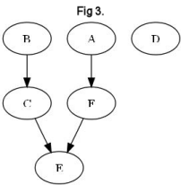
The Standard Method for resolving BeatLoops is very simple. First, examine the smallest BeatLoops and remove all of the BeatWins in those BeatLoops. If longer BeatLoops still remain, the next smallest set is resolved and the process continues until no more BeatLoops survive. Taking the example from the previous page, there is only one BeatLoop, A→B→D→A, and it is considered “3-team loop” as it comprises of 3 teams. Be careful not to count A twice. To resolve the loop, the BeatWins A→B, B→D, and D→A are all removed which leaves us with a new graph (Fig 3). What remains is what we still can determine. A is still better than F and E, but isn't necessarily better than B anymore. B is still better than C and E. We can no longer determine anything about D as both its BeatWin to A and its BeatLoss from B have been removed.

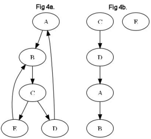
As the set of BeatLoops grows, the resolution must be done in steps to allow for the greatest amount of data to be preserved. Consider the following BeatLoops (Fig 4a):

A→B→C→D→A
B→C→E→B

Since B→C→E→B is the shorter BeatLoop, its BeatWins are removed first. Since B→C existed in the longer BeatLoop, its removal breaks the larger loop and leaves behind C→D→A→B. E loses both its BeatWin and BeatLoss and cannot be graphed in relation to the other teams (Fig 4b). If there is more than one BeatLoop of the same size, all BeatWins in same-sized BeatLoops are removed at the same time before proceeding to longer BeatLoops.

Iterative Method

The Iterative Method is much like the Standard Method, and in the more simple graphs it will give the same result. Where it differs though is that in order to retain more direct BeatWins when all BeatLoops of the same size are considered, any BeatWins that are duplicated are considered for elimination first. Let’s examine the following case first from the Standard perspective, and then the Iterative.

A→B→C→A
A→B→D→A
B→C→E→F→B

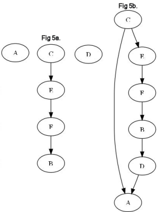
With these three loops, the Standard Method first looks at the two 3-team BeatLoops first. Destroying A→B, B→C, B→D, C→A, and D→A completely rids us of the two smaller BeatLoops, and it breaks the longer BeatLoop leaving us with C→E→F→B while A and D become ambiguous (Fig 5a). At the beginning we had 8 BeatWins and we had to eliminate 5 so we could be left with 3 that are unambiguous. The Iterative method seeks to improve upon the loss of data by removing less.

Instead of taking all BeatWins from all BeatLoops of the same size, the Iterative method looks for the most common BeatWin in the set. Since A→B occurs twice, it will be targeted first. The method assigns a strength to each BeatWin which starts at the number of times the winning team has directly beaten the losing team. For this example, we'll assume each BeatWin is at strength of 1. Since the A→B BeatWin appears twice, we take its strength (1) and divide it by its number of appearances at this BeatLoop size (2). 1/2 = 0.5 and instead of destroying all BeatWins, each is reduced in strength by 0.5 for each time it appears. A→B appears twice and gets reduced by 1 (2 * 0.5) while each of the other BeatWins is reduced by 0.5. When a BeatWin’s strength hits 0, it is removed. In this example, A→B gets removed, while each of the other BeatWins gets to remain, but at 0.5 strength.

Since B→C was not removed the longer BeatLoop still remains and needs to be resolved. This time around, each BeatWin only appears once, but B→C has already been reduced to half strength. Again, we remove as little strength as possible from each until a BeatWin reaches 0. If we reduce all of the BeatWins in the long BeatLoop by 0.5, the B→C BeatWin will be eliminated and the rest of the BeatWins will remain at half strength. At this point all of the BeatLoops will be broken, but this time we will have only destroyed 2 BeatWins while leaving 6 intact and giving us a more complete graph (Fig 5b). In practice, using the Iterative method results in taller, narrower graphs with more interconnectivity which means less ambiguity.

Weighted Method

The biggest difference between the methods used for BeatGraphs and those of other objective statistical systems is that we use as little data as possible to determine the graphs and rankings. The most frequent complaint is that points are not taken into account. Often times there might be a season split between team A and B, but when A won it was by 35 while B only won by 3 in overtime. The argument is that despite the A→B→A BeatLoop, A should be able to retain its BeatWin over B due to the larger margin of victory. Since points are the only determining factor when it comes to who wins or loses (as opposed to yards, first downs, or sacks) we decided it was reasonable to implement a method that uses score data to help determine BeatLoop resolution.

Like the other two methods, BeatLoops are always broken from shortest to longest. Similar to the Iterative Method, the Weighted Method begins by giving each BeatWin a weight. Instead of giving 1 per win though, we give 1 per point. If we take a basic example where A defeats B by 7, B defeats C by 14, and C defeats A by 3, you have a BeatLoop A→B→C→A with BeatWin weights of 7, 14, and 3 in that order. When breaking the BeatLoop, the smallest weight is subtracted from all BeatWins involved in the loop and the BeatWin at 0 is removed. In this case it leaves us with A→B with a weight of 4 and B→C with a weight of 11. Should either of these links be involved in future BeatLoops, their lowered weight will make them more vulnerable to breaking.

The Weighted Method often has a very different interpretation of the results than the other two methods do. It will often allow a team with one fluke blowout to remain higher on the graph than the others would as without support for that win, the others will discard it much more quickly. The benefit of this method however, is that it eliminates the least amount of links and creates the longest and narrowest graphs of the three. This means this method has the least amount of variation between its graph and its respective rankings.